Google Docs Table Conditional Formatting (2025 Guide)

In this tutorial, we will show you exactly how to access Google Docs table conditional formatting in just a few simple steps. Read on to learn more.

Table Conditional Formatting on Google Docs

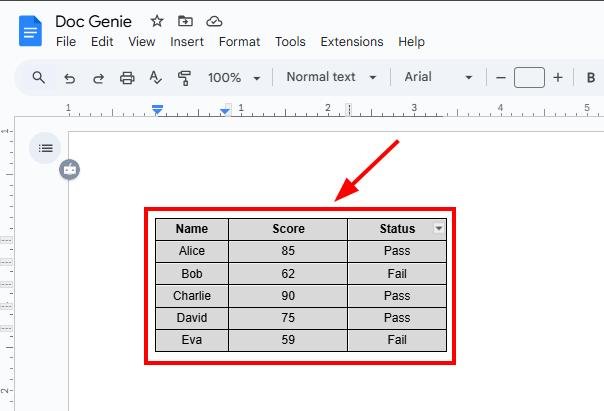
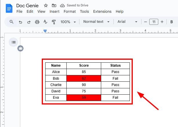
To apply conditional formatting to tables in Google Docs, we will use an example table that includes columns for “Name,” “Score,” and “Status.” Follow the steps below.

1. Highlight and Copy the Pre-Filled Table

Highlight and copy the entire table. Press “Ctrl + C” (Win) or “Cmd + C” (Mac). This prepares your data for conditional formatting in Google Sheets. Make sure to highlight all the cells under your headers as well.

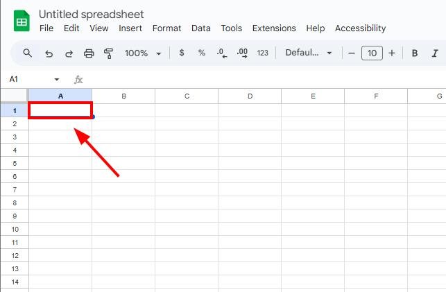
2. Open Google Sheets to Use Conditional Formatting

Since Google Docs does not support conditional formatting directly, open a new Google Sheets document. You will paste the data here for formatting.

3. Paste Your Table Data into Google Sheets

In Google Sheets, paste the table data you copied from Google Docs. Press “Ctrl + V” (Win) or “Cmd + V” (Mac). Ensure the data is correctly aligned in the cells, covering columns A, B, and C.

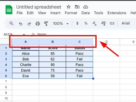
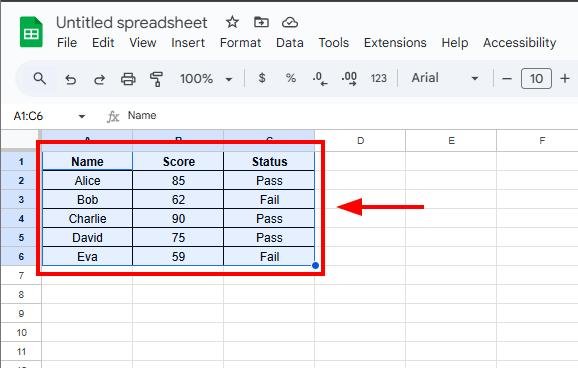
4. Select the Data Range in Google Sheets for Formatting

Click and drag to select the range A1, which includes all names, scores, and statuses. This selection prepares your data for conditional formatting.

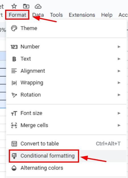
5. Open the Conditional Formatting Menu in Google Sheets

Click on “Format” in the Google Sheets menu and select “Conditional formatting.” This will open a sidebar on the right side of the screen.

6. Set a Conditional Formatting Rule for Low Scores

In the sidebar, choose “Format cells if” 

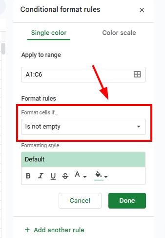
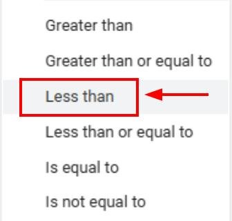
Then, select “Less than.” 

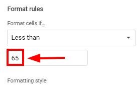
Enter “65” to highlight any scores below 65, marking students who failed.

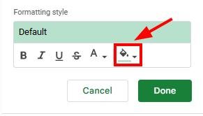
7. Choose a Formatting Style for Failing Scores

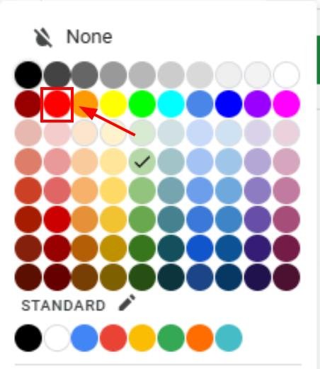
Pick a red background color using the “Fill color” icon.

In our example, we will use this shade of red to make failing scores stand out. 

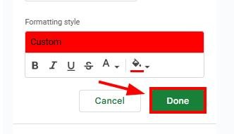
8. Apply the Rule and Review the Changes

Click “Done” to apply the rule. Check your table to ensure all scores below 65 are highlighted correctly. Add more rules if needed to further customize your formatting.

9. Copy the Formatted Table from Google Sheets Back to Google Docs

Once satisfied with the formatting, select the entire table in Google Sheets, copy it, and paste it back into your Google Docs. The visual formatting will transfer, but conditional rules will not be editable in Docs.

We hope that you now have a better understanding of applying Google Docs table conditional formatting. If you enjoyed this article, you might want to check our articles on how to flip a table in Google Docs and how put a table caption on Google Docs.