Pivot Table on Google Docs (The Ultimate Guide for 2024)

In this tutorial, we will show you exactly how to create a pivot table on Google Docs in just a few simple steps. Read on to learn more.

Make a Pivot Table in Google Docs

Follow the steps below to add a pivot table to Google Docs.

1. Highlight the Data Range in Google Sheets

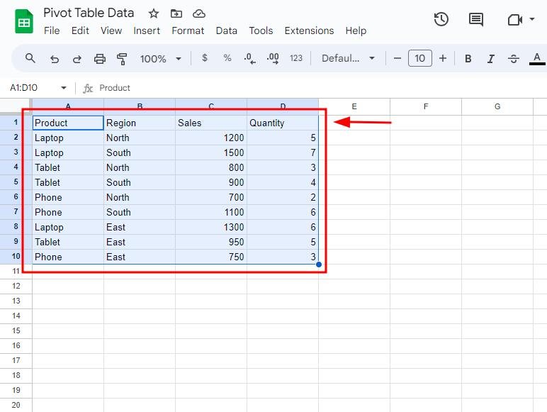
In our example, we have a list of products from cells A2 to A10, each paired with their corresponding region, sales, and quantities spread across cells B2 to D10. We want to use a pivot table to analyze the sales and quantities for each product type.

First, highlight all the data in your Google Sheets file. For example, we will select columns like Product, Region, Sales, and Quantity to ensure we are selecting all relevant information for analysis.

2. Navigate to the Data Menu and Insert a Pivot Table

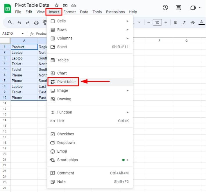
Click on “Insert” in the top menu bar, then select “Pivot table” from the dropdown to create a new pivot table on a separate sheet.

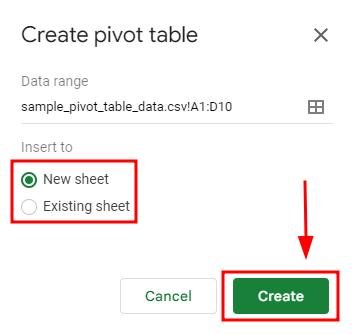
Choose whichever is necessary for your data. In our case, let’s click on “New sheet” under the Insert to section, then click “Create.”

3. Add Products as Rows in the Pivot Table

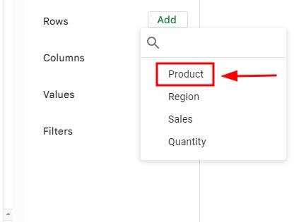
In the Pivot Table Editor on the right side of the screen, click “Add” under Rows.

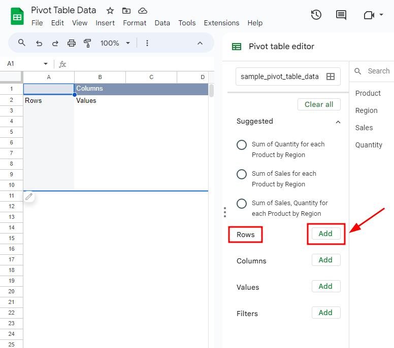
Then select “Product” to create rows for each unique product (Laptop, Tablet, Phone).

4. Add Sales Data as Values to Summarize Sales Amounts

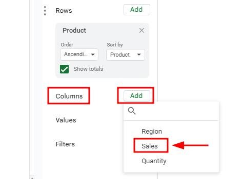
Under the Values section, click “Add” and choose “Sales” to display the total sales value for each product.

5. Add Quantity Data to Values to Display Product Quantities Sold

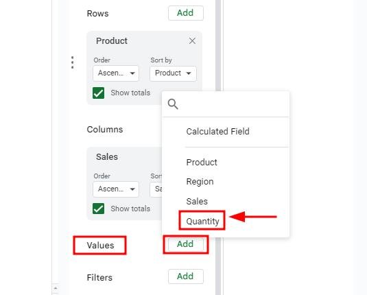
Click “Add” under the Values section and select “Quantity” to add the total quantity sold for each product to the pivot table.

6. Change Summary Type if Needed to Show Sum, Average, or Count

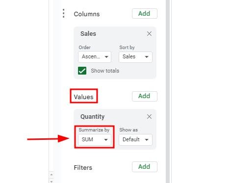
Click the dropdown arrow next to the field under the Values section to change the summary type. Here, we can just use “SUM.” You can use other types, such as Count, Average, etc., for better data analysis.

7. Add a Filter to the Pivot Table to Focus on Specific Data

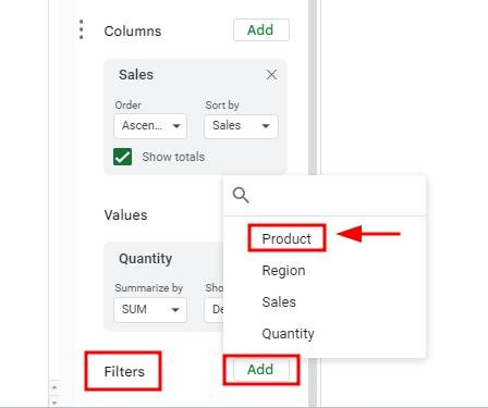
Click “Add” under the Filters section in the Pivot Table Editor and choose a field like “Product” to filter and view specific data points.

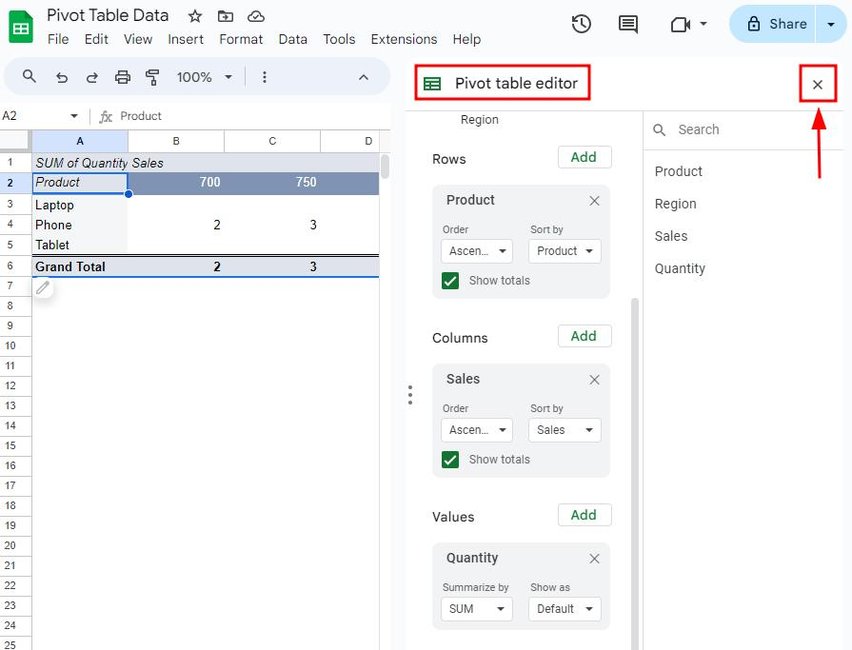
After setting the parameters, you can exit the Pivot table editor by clicking “x.”

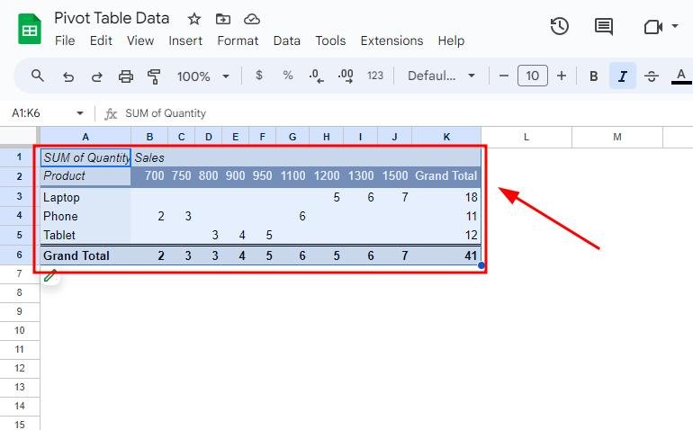
8. Copy the Completed Pivot Table from Google Sheets

After setting up the pivot table, highlight it, then right-click and select “Copy” or press Ctrl + C (Cmd + C on Mac) to copy it to the clipboard.

9. Paste the Pivot Table into Google Docs with Linked Updates

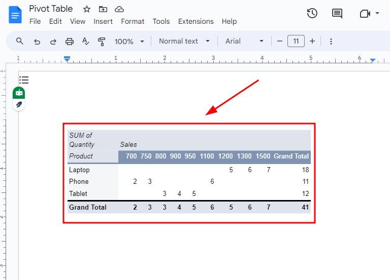
Open Google Docs and place your cursor where you want the pivot table. Right-click and select “Paste” or press Ctrl + V (Cmd + V on Mac). Choose “Link to Spreadsheet” so that updates made in Google Sheets will automatically reflect in Google Docs.

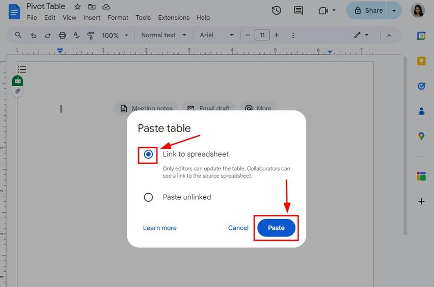
Now, a pivot table is created on your Google Docs file.

We hope that you now have a better understanding of how to set up a pivot table in Google Docs. If you enjoyed this article, you might want to check our articles on how to delete space between tables in Google Docs and how to create a table chart from a template on Google Docs.